Examples
Step-wise Growth Simulation Example
Importance of Stoichiometry
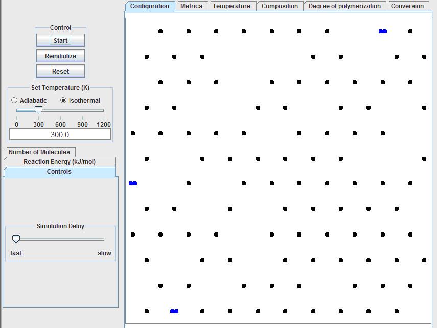
First, run the stepwise growth simulation. The program should look like this after opening:
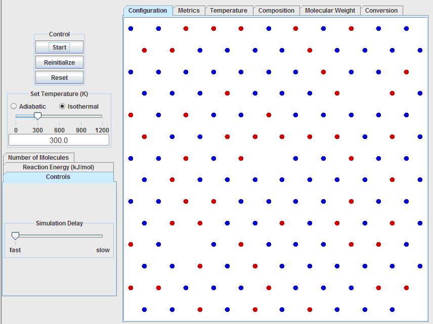
Note that all of the input and control options are located to the left of the visualization window, while all of the output data and calculations are accessible by tabs above the visualization window.
The first input option is to run the simulation under adiabatic or isothermal conditions. The temperature can be controlled by using the slider bar, or by inputting the temperature into the text box. For now, keep the simulation isothermal at 300K.
Below the temperature settings, click on the “Number of Molecules” tab. Set the following:
- Mono-ol: 0
- Mono-acid: 0
- Di-ol: 300
- Di-acid: 200
- Crosslinker: 0
Next, click on the “Reaction Energy” tab (below the “Number of Molecules” tab) and set the reaction energy to 40 kJ/mol. The "fraction heat transfer to solvent" is effectively the heat of reaction that escapes the system. This option allows for the user to simulate different temperature rises for a given bond energy. Otherwise, the simulation would not be able to model strong bonds without a large temperature increase, since both of these quantities would arise from one parameter (the reaction energy). You can set the fraction heat transfer to solvent to 1 to remove the heat of reaction from the system from when two monomers react to help out the thermostat. If you want to run completely adiabatic experiment, you should set this value to 0.
After a short while the visualization window under the “configuration” tab should look something like this:
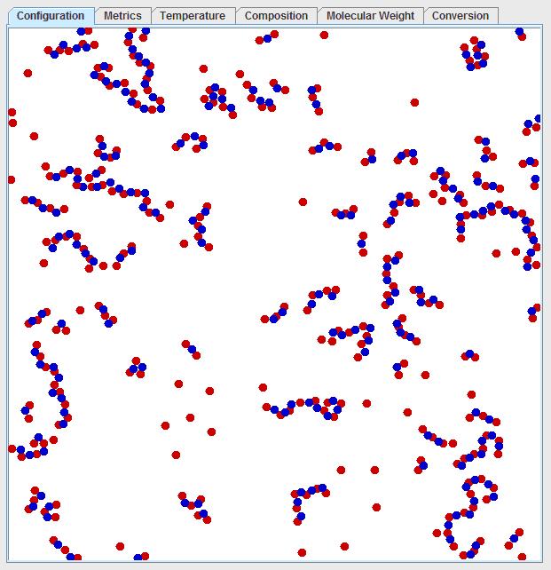
Note that there is significant diversity in the chain lengths. One can predict the average chain length by considering that red dots must bond to blue dots and there is a ratio of 3:2 red dots to blue dots. So, one would expect the average chain to look like: red-blue-red-blue-red. Once this chain forms, the red dots cannot react with other chains that are “end-capped” with red dots, since red dots are in excess. By looking at this average chain, one can see the average chain length would consist of 5 monomers at the maximum conversion. However, few chains have a length of 5 monomers, but for every chain that has 2 more monomers than the average, another chain must have 2 fewer monomers than the average due to the stoichiometry so that the average is maintained. The current temperature and number average degree of polymerization can be viewed under the “metrics” tab. The degree of polymerization as a function of time is plotted in the “Molecular Weight” tab. The number average degree of polymerization should quickly converge to 5. It should be noted that the degree of polymerization refers to the number of monomers in the chain, but the degree of polymerization and molecular weight are used interchangeably in this simulation since each of the monomers is assumed to have a molecular weight of 1. The molecular weight of a real polymer chain would, of course, be the simple sum of all of weights of the units in the chain.
This model illustrates how precise stoichiometric balance is critical to creating high molecular weight polymers, since a slight excess of one reactant can greatly diminish the chain length. For instance, if a ratio of 101 to 100 is considered (a 1% excess of one reactant), then the chain would consist of 100 R-B pairs and then an end-capping R, resulting in a maximum chain length of 201, assuming complete conversion in the absence of any other limiting factors. If the reactants are perfectly balanced, much higher molecular weights are obtainable.
Next, setup the following experiment:
- Mono-ol: 100
- Mono-acid: 0
- Di-ol: 200
- Di-acid: 200
- Crosslinker: 0
Note that the mono-ol (which can only react with one blue dot), has the same end-capping effect as excess alcohol groups, so that the number average degree of polymerization for this experiment also should converge to 5.
Temperature Effects
This model reversibly bonds the molecules together using the reaction energy to indicate both the strength of the bond and the heat of reaction. To see the effects of temperature on a polymerization reaction, set the following:
- Mono-ol: 0
- Mono-acid: 0
- Di-ol: 500
- Di-acid: 500
- Crosslinker: 0
If the simulation is run isothermally at 300K, note that long chains are obtainable. However, if the simulation is run adiabatically starting at 300K with the “fraction heat transfer to solvent = 0” (again, found under the Reaction Energy tab), then the temperature increases dramatically, which will cause depolymerization (the chain starts to break apart) and can limit the maximum molecular weight obtainable. The user can monitor the current temperature under the “Metrics” tab or the temperature history under the “Temperature” tab.
This is a realistic concern as polymerization reactions can be very exothermic. The unrealistic aspect of this simulation is that when a real polymer thermally degrades, it usually forms a myriad of degradation products which cannot re-polymerize, whereas in this simulation, the chains break to reform the monomers which can react again.
Gelation
To model gelation, again set the simulation to run isothermal at 300K.
Below the temperature settings, click on the “Number of Molecules” tab. Set the following:
- Mono-ol: 0
- Mono-acid: 0
- Di-ol: 700
- Di-acid: 400
- Crosslinker: 200
Next, click on the “Reaction Energy” tab (below the “Number of Molecules” tab) and set the reaction energy to 40 kJ/mol. Set the fraction heat transfer to solvent to 1.000.
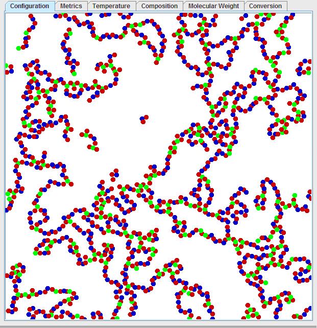
After a high conversion is reached, which may take some time, you should observe a polymer chain which moves from one end of the periodic boundary condition to the other from top to bottom or left to right as seen below:
By tracing along the polymer chain, one can observe regions where the polymer enters from the bottom and leaves on the same point on the top. This can be better observed by left clicking on the visualization window, then pressing “1” to see the mosaic view:
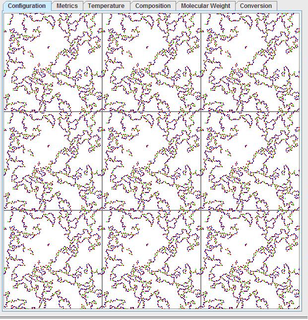
Pressing “0” will return to the original window. Considering the periodic boundary condition, this would mean the polymer has an infinite molecular weight. This is not just an artifact of the periodic boundary condition, but rather it is a real effect known as gelation! Gelation is the formation of this interconnected structure, where the polymer ceases to be a high molecular weight fluid and becomes a solid of infinite molecular weight. A common household analogy would be that of gelatin, where the dissolved gelatin molecules will cross-link over time to become an increasingly viscous fluid and then suddenly become a solid.
Model Output
There are several ways of visualizing the output of the simulation. Across the top, the “configuration” tab shows the visualization of the polymerization, the “Metrics” tab gives the current data, the “Temperature” tab give the temperature history, the “Composition” tab gives a histogram of the chain lengths, the “Molecular Weight” tab shows the number-average and weight-average degrees of polymerization as functions of time, and the “Conversion” tab shows the fraction of alcohol and acid groups that have been consumed over time (Note, there will be two separate lines if the reactants are imbalanced). One of the most important features of these tabs is that the user can click on a tab, such as “Conversion”, then right-click on the graph to get a table of the raw data. This data table can then be copied and then imported into a spreadsheet so that the user can perform his/her own calculations. For instance, a user can right-click on the conversion, copy and paste the data into Microsoft Excel, calculate the amount of unreacted groups from the conversion over time, and then model the kinetics of the reaction and determine the reactions rate constants and order. The order of the reaction determined can then be compared to what the user might expect from theory.
Free Radical Chain Addition Example
First, run the free radical chain addition simulation. The program should look like this after opening:
Initiators
Again, set the simulation to run isothermally at 300K. Then click on the “Number of Molecules” tab on the left to enter:
- Initiator: 20
- Monomers: 0
Next, click on the “Reaction Energy” tab and set the following reaction energies:
- initiator-initiator: 15 kJ/mol
- radical reaction: 40 kJ/mol
The first energy is the energy that holds the initiator together, the second energy is that of the monomer addition. Set the fraction heat transfer to solvent to 1.000 and the combination probability to 0.000.
Start the simulation. Note each of pair of blue dots represent one initiator. Over time, the thermal energy will overcome the bonding energy of the initiator, splitting the initiator into two free radical species (shown in green). This will occur more often if the bonding energy is lower, or if the temperature is higher. Hence, a common strategy for initializing polymerization reactions is to mix the polymer with the initiator, then heat the mixture to activate the free radicals when the engineer wishes to begin polymerization.
Initiator to Monomer Ratio
Now, set the simulation to run isothermally at 300K. Then click on the “Number of Molecules” tab on the left to enter:
- Initiator: 50
- Monomers: 500
Run the simulation and note the steps which take place. First, the initiator splits to form two free radicals. The free radical then bonds to a monomer (black). The monomer then becomes active (red) and will bond to another monomer. After bonding with the monomer, the previous monomer loses its activity (and turns grey), while the newly added polymer becomes reactive (red). The chain then propagates by adding one monomer at a time to the chain. (Hence, the name chain addition) The polymerization stops when to active chain ends collide. This termination reaction can either result in the growing chains combining (termination by combination) or in the chains reacting by transferring the radical and killing the activity of both chains (termination by disproportionation). The probability of combining is set under the “Reaction Energy” tab. If two active ends collide but do not combine, the model terminates the polymerization by disproportionation. Note that if you reinitialize the polymerization and set the combination probability to 1, the number-average molecular weight achieved at complete conversion will be approximately double the value obtained when the probability is 0.
Next, click on the “Reaction Energy” tab and set the following reaction energies:
- initiator-initiator: 0 kJ/mol
- radical reaction: 40 kJ/mol
Setting the initiator bonding energy to 0 will allow for instant disassociation of the initiator, speed up the polymerization, and make some of the results more repeatable. Set the fraction heat transfer to solvent to 1.000 and the combination probability to 0.000. At high conversions, the number-average molecular weight should be near 5, because this value can be calculated by dividing the number of monomers (500) by the number of free radical initiators (50 x 2). The number found in the simulation may be slightly higher, since not all of the initiators may have formed growing chains. Again, if the same simulation is run with a combination probability of 1, then the number average molecular weight should approximately double to 10. Note that increasing the amount of initiator should increase the rate of conversion, but every time the amount of initiator is doubled, the resultant molecular weight is cut in half.
Note on Temperature Effects
Polymers made from free radical chain addition are also vulnerable to thermal degradation, but the depolymerization reactions are not allowed in this model. However, under adiabatic conditions, this type of reaction is similarly auto-accelerating. One positive thermal feedback loop is that the heat of reaction causes faster movement of molecules, allowing for faster reactions. In addition, this increased heat will allow more initiators to split to form free radicals which will form more propagating chains, which will generate more heat. Further polymerization makes the solution more viscous and unable to dissipate heat, which exacerbates the temperature rise. This increase in viscosity can also reduce the rate of termination in what is known as the “gel effect.” This auto-acceleration is also known as the Trommsdorf effect, which is important safety issue, since the temperature rise in the presence of monomer or solvent could result in an explosion.