Tuning the Model Parameters

Background

The applet supplies a set of parameters for MW, σ, ε, and λ that roughly approximate Xenon, but we have no indication of how reliable they are. (FYI: notation is listed on the Basic Layout page.) For starters, let’s assume the values of σ and λ are reliable, but we want to check the value of ε. Referring to the steam tables, we see that the liquid density is roughly 1000 times higher than the vapor density at the normal boiling temperature. We can use this observation along with assuming that the vapor is nearly an ideal gas(ie. ZVap≈PVig/RT=1). This gives an estimate of ZLiq=P*VLiq/RT≈0.001. So we simply need to set the density to the experimentally known saturated liquid value, then simulate the pressure for a few temperatures, and plot ZLiq vs. temperature and extrapolate to ZLiq≈0. FYI: This procedure can be slightly improved if we plot ZLiq vs. 1000/T, because then we obtain roughly linear behavior. In fact, reciprocal temperature is almost always more convenient than temperature when analyzing thermodynamic behavior. Armed with this plot, we can evaluate the quality of ε. If T(@ZLiq=0) = Tb, then our value of ε is acceptable.

The values of the parameters are set on the "potential" tab. There you will see that MW=131g/mol, σ=0.4nm, ε=1000J/mol, and λ=2.0. If we increase the value of ε, the molecules should become "stickier," requiring a higher temperature to boil. At even higher temperatures, the kinetic energy at very high temperature can overwhelm the potential energy. When $\epsilon/RT<0.01$, the potential energy becomes practically negligible relative to the kinetic energy. Can you think of another name for a square well potential model with negligible potential energy (ie. ε=0)? Look back at Figure 1. Do you see that the square well model becomes the hard sphere model when ε=0? That's actually quite convenient because we can simulate hard spheres relatively quickly. Better yet, we can just calculate it using the CS model since previous HS simulations have demonstrated the reliability of the CS model.

So, let's review. A plot of ZLiq vs. 1000/T is roughly linear. The y-intercept of that plot is given by the HS model. So we really need just one more point on that line to nail down our estimate of the boiling temperature. Of course, our accuracy would be improved if we simulated points closer to Zliq=0.

Finally, suppose the estimate of Tb obtained in this way does not agree with the experimental value. Then what? Well, we know that Tb increases with increasing ε. And, to the extent that ZLiq is linear, a plot of ZLiq vs. ε/RT should be similar. So we don't need to re-simulate. We just need to find the value of ε that corrects the slope of the curve. That is,

ε(opt)/ε(sim) = Tb(expt)/Tb(sim).

Problem Statement

Determine the density of saturated liquid Xenon at its normal boiling temperature using the resources at webbook.nist.gov. Simulate square well spheres at that density using λ=2.0 and at a temperature of 200, 250, 500, 750K. Use this analysis to determine a value for ε that matches the boiling temperature of Xenon and compare it to the default value of 1000J/mole.

Solution

Referring to webbook.nist.gov, the density at 165K is 22.41 mol/L. We can also simulate a table of Z factors from 175-750K. For the SW fluid, we obtain the tabulated Z factors at 0.02241 mol/cm3 (364 molecules). FYI: $η=0.02241\*602E21 π0.4^3/(6\*1E21)=0.452$.

SW results at $\eta = 0.452$, $\lambda = 2.0$, ε = 1000J/mol, $\sigma = 0.4nm$, $\rho = 22.41 mol/L$.

T(K)	t(ps)	t(min)	P(MPa)	U(J/mol)	Z
205.6 ± 0.46	311	35	3.32 ± 1.1	-1458 ± 0.48	0.086
220.6 ± 0.52	155	15	24.76 ± 1.8	-1451 ± 0.74	0.602
490.6 ± 0.34	212	25	505.9 ± 2.5	-1402 ± 0.27	5.535
763.8 ± 0.65	168	35	993.7 ± 1.7	-1389 ± 0.78	6.983
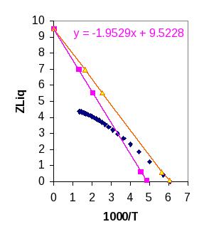
∞ (HS, 300)	123	2	532.1 ± 1.4	0	9.520

The trendline indicates that Tb(sim)=205.1K, but Tb(expt)=165. So a better value for ε would be ε=1000*165/205 = 805J/mol. We do not need to re-simulate the system. At T=∞, the HS value will still prevail and we know what the shift will be at Tb. This leads to the orange line for the simulation data with the new value of ε.

Having matched the boiling temperature along the x-axis, it becomes more apparent that the slope and y-intercept are deficient. This suggests that another parameter may be wrong, but which? We could obtain a reasonable representation at more common conditions if the y-intercept were 6.6. Does a lower intercept indicate a higher or lower packing fraction? Which parameter (σ or λ) could be varied to alter the packing fraction (the space occupied by molecules) while maintaining a density of 22.41mol/L? What exact value of η would permit you to match ZHS = 6.0? (Hint: if the CS equation gives accurate values for ZHS(η), do you really need to simulate iteratively to answer this question?)

Homework: Problem 2.6

In case you are wondering, the curvature in the experimental data at high temperature results from the softness of the interactions between real molecules. The square well model assumes that the repulsive energy is infinite at r < σ, so it cannot characterize this softness accurately. Returning to the truck analogy, slamming a truck into a cliff at Mach 3 might make a non-negligible dent. The square well approximation oversimplifies slightly, but 750K and 611MPa are uncommon conditions. Many applications may be studied with the square well model at more modest conditions.

∞ ε π σ λ η β ε ρ ± ≡ ² ³ ≈